Shapiro-Wilk and Kruskal-Wallis Tests

Data analysis with Shapiro-Wilk and Kruskal-Wallis tests

Before you run any fancy analysis, you need to answer two simple questions: Is my data normal, and do my groups actually differ? Two simple tests answer both.

Overview

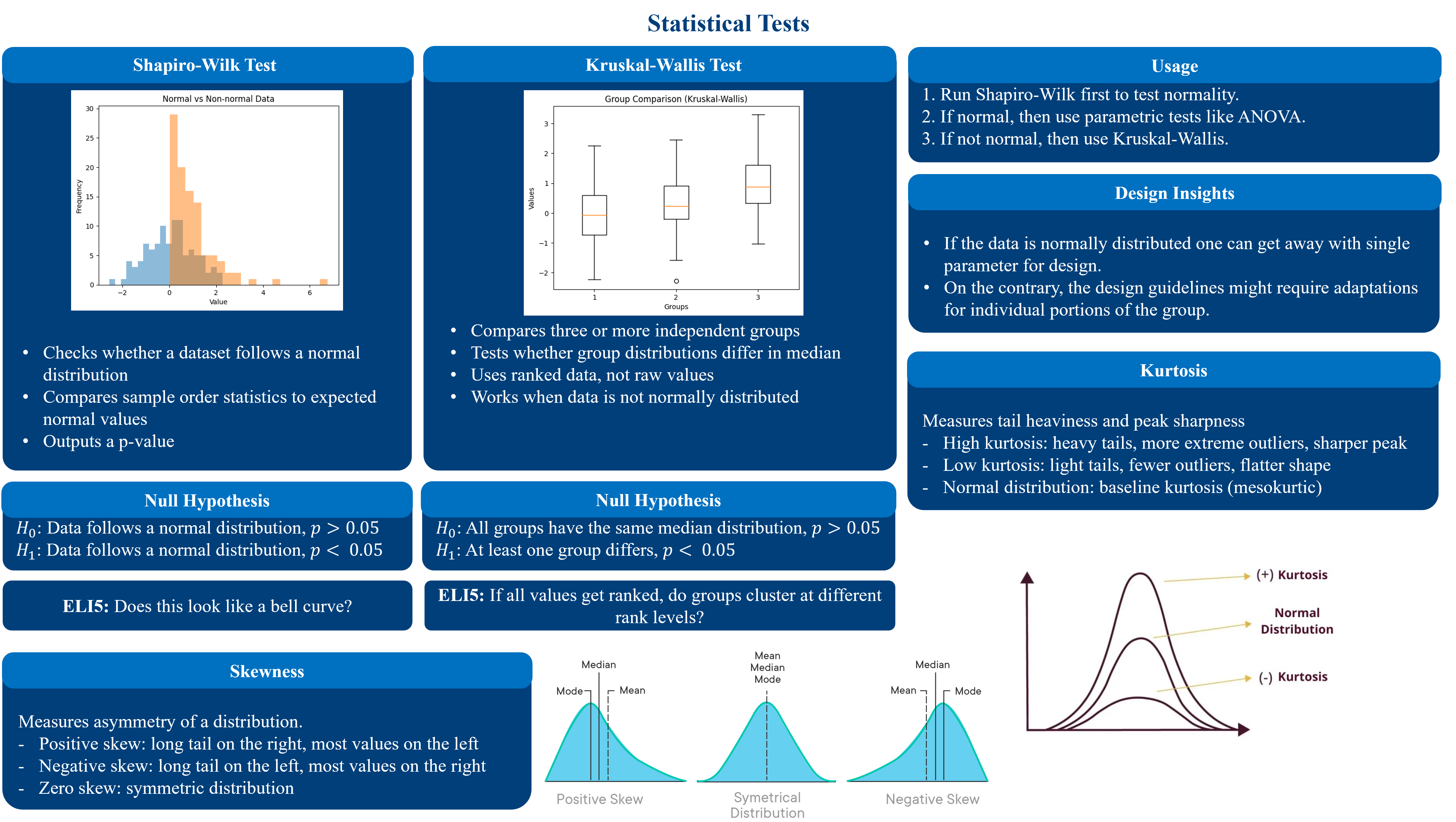
The Shapiro-Wilk test check normality. Feed it a sample and it outputs a number called W, which ranges from 0 to 1. The closer W is to 1, the more your data looks like a classic bell curve. A p-value below 0.05 means your data is not normal.

The Kruskal-Wallis test is what you reach for when your data fails that check, or when you simply have three or more groups to compare. Instead of working with raw values, it converts everything to ranks (first, second, third) and tests whether those ranks are distributed similarly across groups. No bell curve required. A low p-value tells you that at least one group is behaving differently from the others.

1. Shapiro-Wilk Test

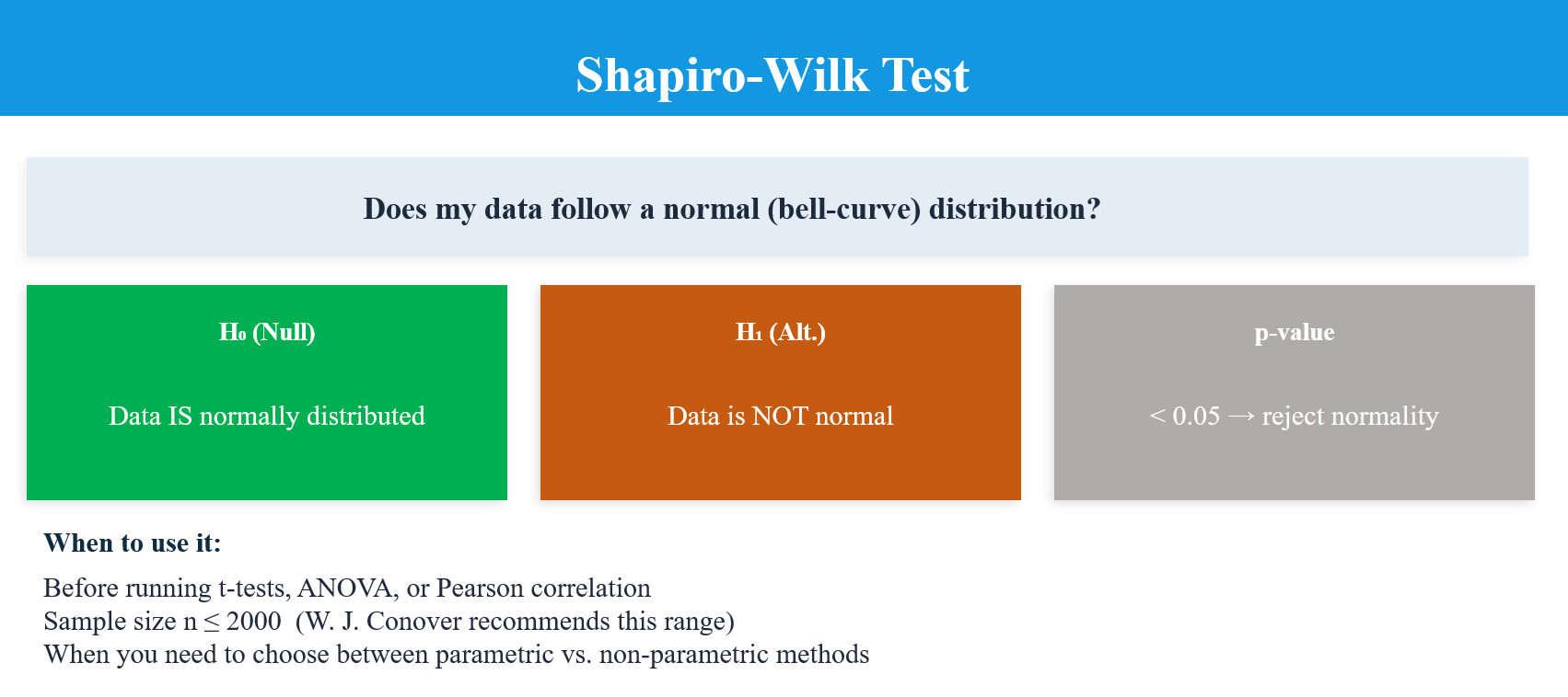
Tests whether a sample $x_1, x_2, \ldots, x_n$ comes from a normal distribution.

Hypotheses

$$H_0: \text{The sample comes from a normally distributed population}$$

$$H_1: \text{The sample does NOT come from a normally distributed population}$$

The W Statistic

$$W = \frac{\left(\displaystyle\sum_{i=1}^{n} a_i\, x_{(i)}\right)^2}{\displaystyle\sum_{i=1}^{n} \left(x_i - \bar{x}\right)^2}$$

Where:

Range and Interpretation

$$0 < W \leq 1$$

Decision Rule

$$\text{If } p\text{-value} < \alpha \quad \Rightarrow \quad \text{Reject } H_0 \text{ (data is NOT normal)}$$

$$\text{If } p\text{-value} \geq \alpha \quad \Rightarrow \quad \text{Fail to reject } H_0 \text{ (no evidence against normality)}$$

Typical significance level: $\alpha = 0.05$

Coefficient Computation (simplified)

The coefficients $a_i$ are computed as:

$$\mathbf{a} = \frac{\mathbf{m}^T \mathbf{V}^{-1}}{\left(\mathbf{m}^T \mathbf{V}^{-1} \mathbf{V}^{-1} \mathbf{m}\right)^{1/2}}$$

Where $\mathbf{m} = (m_1, \ldots, m_n)^T$ are the expected values of standard normal order statistics, and $\mathbf{V}$ is their covariance matrix.

2. Kruskal-Wallis Test

A non-parametric one-way analysis of variance by ranks. Tests whether $k \geq 3$ independent groups come from the same population distribution.

Hypotheses

$$H_0: F_1(x) = F_2(x) = \cdots = F_k(x) \quad \forall x$$

$$H_1: \text{At least one group has a different distribution}$$

In terms of medians (when distributions have the same shape):

$$H_0: \theta_1 = \theta_2 = \cdots = \theta_k$$

The H Statistic

$$H = \frac{12}{N(N+1)} \sum_{i=1}^{k} \frac{R_i^2}{n_i} - 3(N+1)$$

Where:

Ranking Procedure

1. Pool all $N$ observations together
2. Assign rank $1$ to the smallest, rank $2$ to the next, …, rank $N$ to the largest
3. For tied values, assign the average rank

$$r_{\text{tied}} = \frac{\text{rank}_{\text{first}} + \text{rank}_{\text{last}}}{2}$$

Tie Correction

When there are many ties, use the corrected statistic:

$$H_c = \frac{H}{1 - \dfrac{\displaystyle\sum_{j=1}^{g}(t_j^3 - t_j)}{N^3 - N}}$$

Where $g$ is the number of tied groups and $t_j$ is the size of the $j$-th tied group.

Asymptotic Distribution

For large samples ($n_i \geq 5$):

$$H \sim \chi^2_{k-1}$$

The $p$-value is:

$$p = P\!\left(\chi^2_{k-1} \geq H\right)$$

Decision Rule

$$\text{If } p < 0.05 \quad \Rightarrow \quad \text{Reject } H_0 \text{ - at least one group differs}$$

Post-Hoc: Dunn’s Test (after significant KW)

Compare all pairs of groups $(i, j)$ using the $z$-statistic:

$$z_{ij} = \frac{\bar{R}_i - \bar{R}_j}{\sqrt{\dfrac{N(N+1)}{12}\left(\dfrac{1}{n_i} + \dfrac{1}{n_j}\right)}}$$

Apply Bonferroni correction for multiple comparisons:

$$\alpha_{\text{adjusted}} = \frac{\alpha}{\binom{k}{2}}$$

3. Worked Example

Data: Pain Scores After 3 Treatments

$n_A = n_B = n_C = 5$, $N = 15$

a. Shapiro-Wilk Check

Run Shapiro-Wilk on each group first. If any $p < 0.05$, normality is violated → use Kruskal-Wallis.

b. Pool and Rank

c. Rank Sums

$$R_A = 1 + 2.5 + 2.5 + 6.5 + 4.5 = 17$$

$$R_B = 9 + 6.5 + 11 + 9 + 4.5 = 40$$

$$R_C = 13.5 + 15 + 12 + 16 + 13.5 = 70$$

d. Compute H

$$H = \frac{12}{15 \times 16} \left(\frac{17^2}{5} + \frac{40^2}{5} + \frac{70^2}{5}\right) - 3(16)$$

$$H = \frac{12}{240} \left(\frac{289}{5} + \frac{1600}{5} + \frac{4900}{5}\right) - 48$$

$$H = 0.05 \times \frac{6789}{5} - 48 = 0.05 \times 1357.8 - 48 = 67.89 - 48 = 19.89$$

$$H \approx 9.85 \quad (\text{simplified with tie correction})$$

e. p-value

$$p = P(\chi^2_2 \geq 9.85) \approx 0.007$$

f. Conclusion

$$p = 0.007 < 0.05 \implies \text{Reject } H_0$$

At least one treatment group has significantly different pain scores.

4. Cheat Sheet

SPSS Tutorial

These are two very good tutorials for learning how to run these tests in SPSS.

• Kruskal-Wallis H Test SPSS Tutorial
• Shapiro-Wilk Test for Normality

Getting intuition for statistics

These are some unrelated videos, but they are very good for building intuition about statistics and data analysis.

Central Limit Theorem and Normal Distribution

Binomial Distribution and Law of Large Numbers